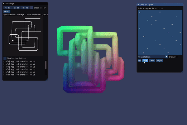
Grid Diagrams

➰ A program for manipulating and playing with knot diagrams.

Description

Grid Diagrams

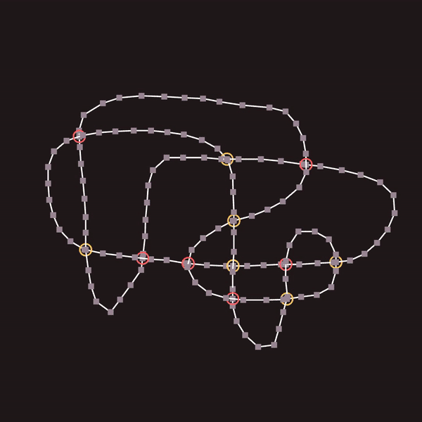
One interesting way to represent knots (a presentation of the knot) is via a so-called n x n grid diagram. The contents of each grid cell is x, o, or “blank.” A grid diagram has the property that every row and column has exactly one x and one o. We can construct the knot corresponding to a particular grid diagram using the following algorithm:

1. In each column, connect each x to the corresponding o
2. In each row, connect each o to the corresponding x
3. Whenever a horizontal segment intersects a vertical segment, assume that the vertical segment passes over the horizontal segment (i.e. a grid diagram only consists of over-crossings)

In practice, we can traverse the diagram by starting with the x in the left-most column. We connect this to the o in the same column. Now, we “switch directions” and move to the x in the corresponding row. We continue in this fashion (alternating between rows and columns) until we reach the grid cell from which we started. Upon completion, we will have created a closed, polygonal curve that is a geometric representation of the knot. However, we haven’t done anything with the crossings in the diagram. Figuring out where each intersection occurs is straightforward, since all of these points will necessarily lie on the grid. After doing so, we “lift” these intersection points along the positive z-axis by 1 grid unit. The exact amount is arbitrary: we simply want to make sure that the grid starts in a valid state with no self-intersections (this is necessary for the physics simulation to behave properly, as described below).

Refinement

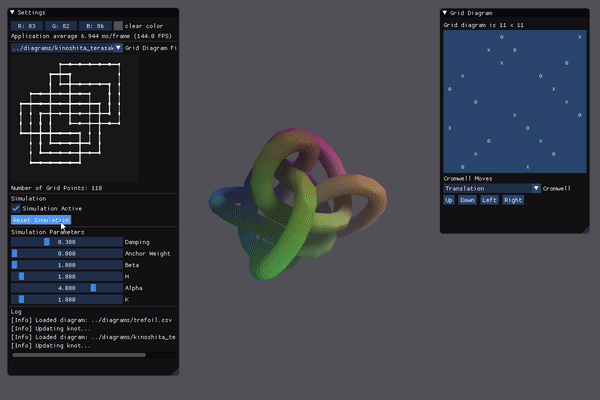
Following the procedure outlined above results in a piecewise linear link (polyline). To obtain a “smoother” projection of the knot (one without sharp corners), we need to perform some form of topological refinement, taking care to not change the underlying structure of the knot. Following Dr. Scharein’s thesis (link below), each vertex of the polyline is treated as a particle in a physics simulation. Adjacent particles are attracted to one another via a mechanical spring force. Non-adjacent particles are repelled from one another via an electrostatic force, which (in practice) prevents segments from crossing over or under one another. Additionally, we perform intersection tests between all pairs of non-neighboring line segments to prevent any “illegal” crossings. This is why we “lift” vertices at all of the crossings when we pre-process the grid diagram.

The relaxation is fairly dependent on both the settings of the simulation parameters as well as the density of the underlying polygonal curve. One TODO item is to investigate more robust ways of resampling a polyline.

Before the knot is rendered, a path-guided extrusion is performed to “thicken” the knot. At each vertex along the polyline, a coordinate frame is established by calculating the tangent vector and a vector orthogonal to the tangent. Then, a circular cross-section is added at the origin of this new, local coordinate system. Adjacent cross-sections are connected with triangles to form a continuous, closed “tube.” To avoid jarring rotations, parallel transport is employed. Essentially, each successive coordinate frame is calculated with respect to the previous frame. This ensures that the circular cross-sections smoothly rotate around the polyline during traversal.

Cromwell Moves

The Cromwell Moves are similar to the Reidemeister Moves, specifically applied to grid diagrams. They all us to obtain isotopic knots, i.e. knots that have the same underlying topology but “look” different. This gives us a way to systematically explore a given knot invariant.

There are 4 different Cromwell moves:

1. Translation: a move that cyclically translates a row or column in one of four directions: up, down, left, or right
2. Commutation: a move that exchanges to adjacent, non-interleaved rows or columns
3. Stabilization: a move that replaces an x or o with a 2x2 sub-grid
4. Destabilization: a move that replaces a 2x2 sub-grid with a single x or o (the opposite of a stabilization)

More information can be found in the following poster titled “Randomly Sampling Grid Diagrams of Knots.”

To Use

All grid diagrams must be “square” .csv files (the same number of rows as columns). Each row and column must have exactly one x and one o: all other entries should be spaces (“blank”). The grid diagram will be validated upon construction, but the program will exit if one of the conditions above is not met. An example grid diagram for the trefoil knot is shown below:

x, ,o, , 
 ,x, ,o, 
 , ,x, ,o
o, , ,x, 
 ,o, , ,x

New diagrams can be added to the diagrams folder at the top-level of this repository. A bunch of example diagrams can be found in the follow paper written by Wutichai Chongchitmate titled “Classification of Legendrian Knots and Links.”

Future Directions

Converting grid diagrams into 3D curves is not something that I came across directly in my research. Although my method of “lifting” the curve at each of the crossings works, it seems rather “hacky.” An alternate representation uses cube diagrams, which are inherently 3D, and therefore, would always start in a valid configuration. Unfortunately, I wasn’t able to find nearly as much information about cube diagrams in my research, so for now, I leave that as an open topic of research.

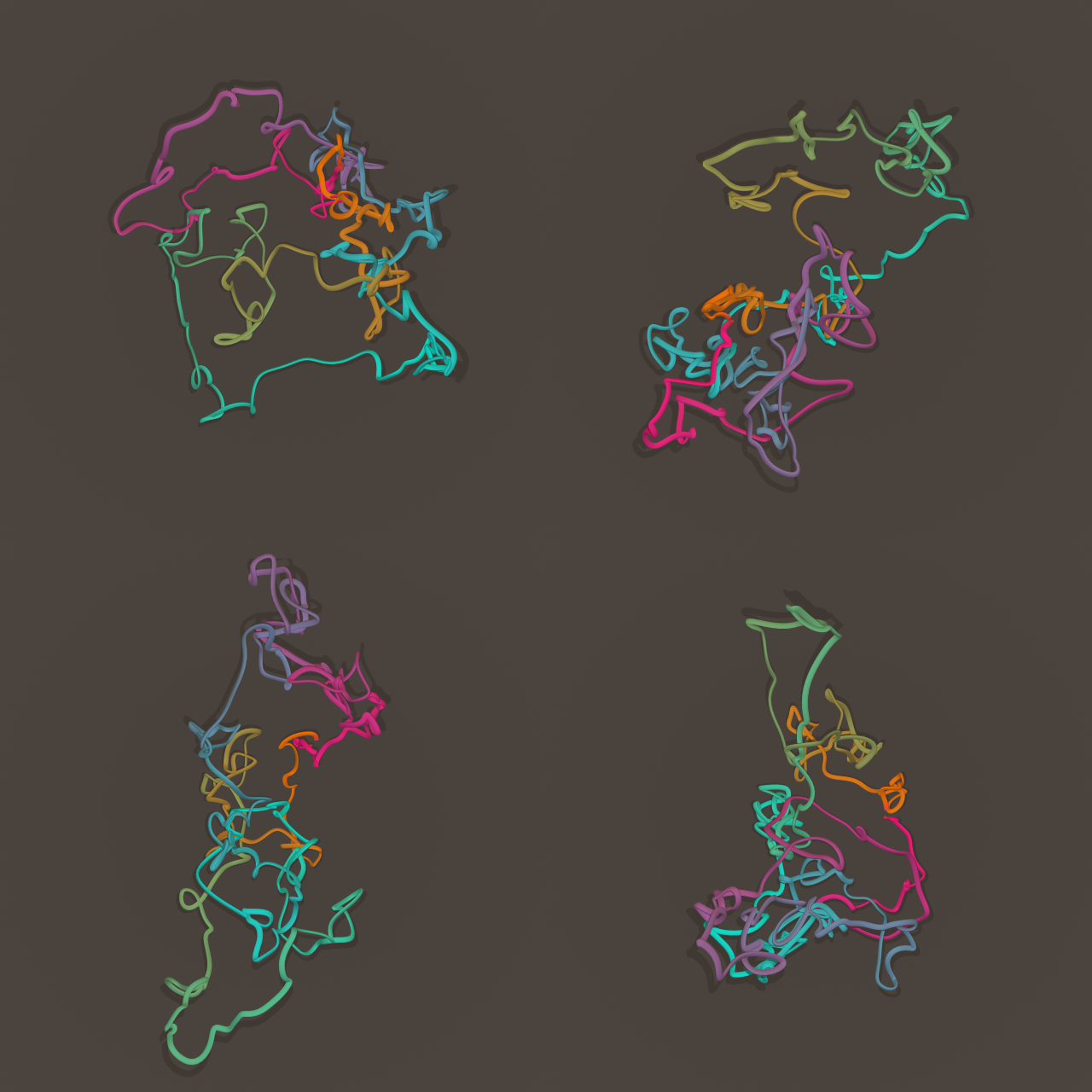
One interesting area of study in the field of knot theory is that of random knot generation. This turns out to be quite a challenging problem. How do we generate a curve that is actually knotted? Moreover, how do we prove that it is, in fact, knotted? Dr. Jason Cantarella has done significant research into this topic, which I would love to explore. Early on, I created a “naive” algorithm for randomly generating grid diagrams, but the vast majority of these diagrams resulted in the unknot (or knots with more than one component). Some of the randomized diagrams output from that program are shown below. This observation prompted me to explore this problem further.

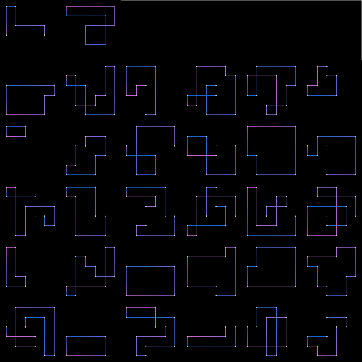
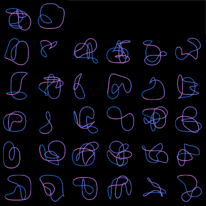
Fundamental to the problem of random knot generation is representation. More specifically, what are all of the different ways that we can represent knots (mathematically, or otherwise)? Clearly, grid diagrams and cube diagrams are two forms of representation, but there are others. One interesting algorithm is the so-called hedgehog method, which produces random, closed polygonal curves. Some examples of curves generated via my (naive) implementation of the hedgehog method are shown below. Knots can also be represented as planar graphs, which leads to the question: how can we generate random, 4-valent planar graphs? My initial research yielded blossom trees, which are essentially trees with additional edges that are used to form closed loops in the graph. Blossom trees can be used to sample random planar graphs.

Beyond this, there are also other ways to catalog and diagram knots: Dowker codes, Conway notation, Gauss codes, braid representations, among others. Dr. Scharein (mentioned below) implemented a “tangle calculator” for building knots from small, molecular components called “tangles.” He also implemented a tool for “drawing” knots by hand, which is something that I explored as well. One challenge with such a tool is: how does the user specify under-/over-crossings? In the prototype that I created (shown below), the crossings would simply alternate whenever the user crossed an existing strand. There is a lot to explore here as well!

Finally, the pseudo-physical simulation used in this program is just one way to perform topological refinement. Dr. Cantarella has also explored this topic with his “ridgerunner” software, which can “tighten” a knot via a form of constrained gradient descent. Are there other ways to accurately “relax” knots?

Credits

This project was largely inspired by and based on previous work done by Dr. Robert Scharein, whose PhD thesis and software were vital towards my understanding of the relaxation / meshing procedures. I would also like to thank Patrick Plunkett (@drknottercreations on Instagram) who sent me many inspiring papers and links throughout this project.

back