Hopf

🧣 A graphical program for exploring the Hopf fibration.

Description

The Hopf fibration is a mapping from S3 to S2 discovered by Heinz Hopf in 1931. Confusingly (at least for me), S3 actually refers to the sphere (or hypersphere) in 4D space. Similarly, S2 refers to the sphere that we are most familiar with in 3D space. To quote Wikipedia: “Hopf found a many-to-one continuous function (or ‘map’) from the 3-sphere onto the 2-sphere such that each distinct point of the 2-sphere is mapped to from a distinct great circle of the 3-sphere.”

The first thing to understand is that a great circle is essentially a “slice” of a sphere that passes through its center. It is difficult to visualize what a great circle on the surface of a 4-dimensional sphere looks like, but luckily, we don’t have to. Each of these great circles in the domain of the mapping function forms a “fiber” that we can project down to 3-space. Doing so results in a beautiful structure of nested shapes that appear to be intricately woven together.

To be more specific, the mapping treats each point on the surface of S3 <a, b, c, d> as a unit quaternion r = a + b*i + c*j + d*k (a unit quaternion is one whose norm is 1). Next, we pick a “principal point” on S2: in the literature, this is usually a unit vector along one of the standard basis vectors, i.e. <1, 0, 0>. The fiber for any point p on S2 consists of all of the unit quaternions that send the principal point p0 to p, via a rotation in 3-space.

For example, let p be the principal point such that p = p0. The fiber corresponding to p is the set of all unit quaternions <cos(t), sin(t), 0, 0> for any scalar value t. Each of these quaternions, when applied to p0, result in p0 itself. So the question becomes: given any point p on S2, how do we find the set of all quaternions that rotate the principal point to p (i.e. the fiber on S3 that corresponds to p)?

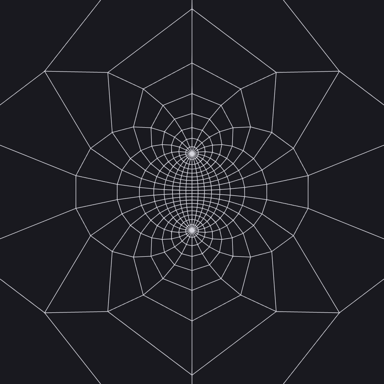
To actually visualize the fibers of the Hopf fibration, we use a stereographic projection that projects points in 4-space into 3-space. Because each fiber is a circle embedded in 4-space (as explained above), its stereographic projection will similarly be a circle in 3-space. For reference, the stereographic projection of S2 and S3 are shown side-by-side below.

To Use

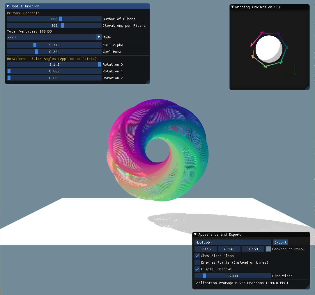
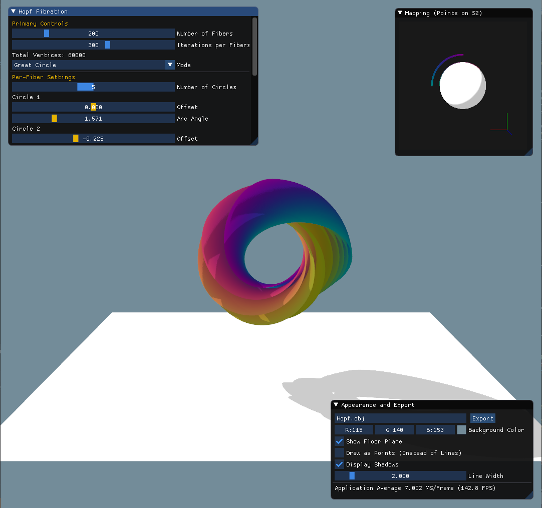
Upon launching the application, you should see three separate UI panels labeled:

• Hopf Fibration: contains controls for adjusting the number of fibers, mode selection, etc.
• Mapping (Points on S2): renders the active base points on the surface of a sphere in 3-space
• Appearance and Export: contains some basic settings for adjusting the appearance of the model as well as a button for exporting the model as an .obj file

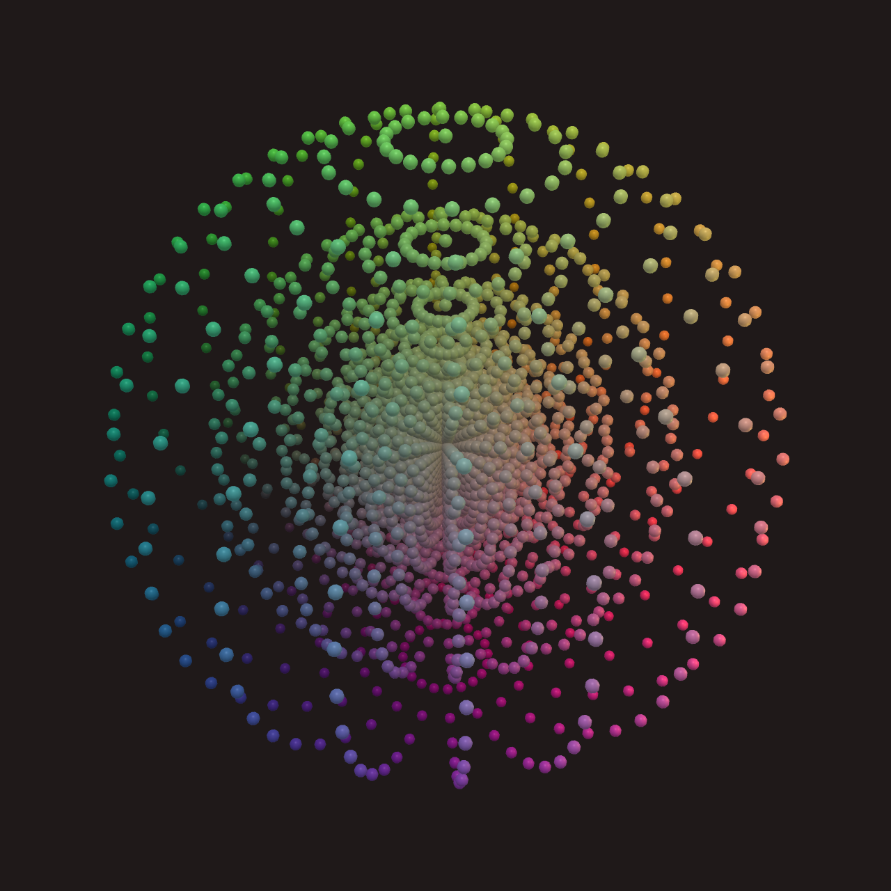
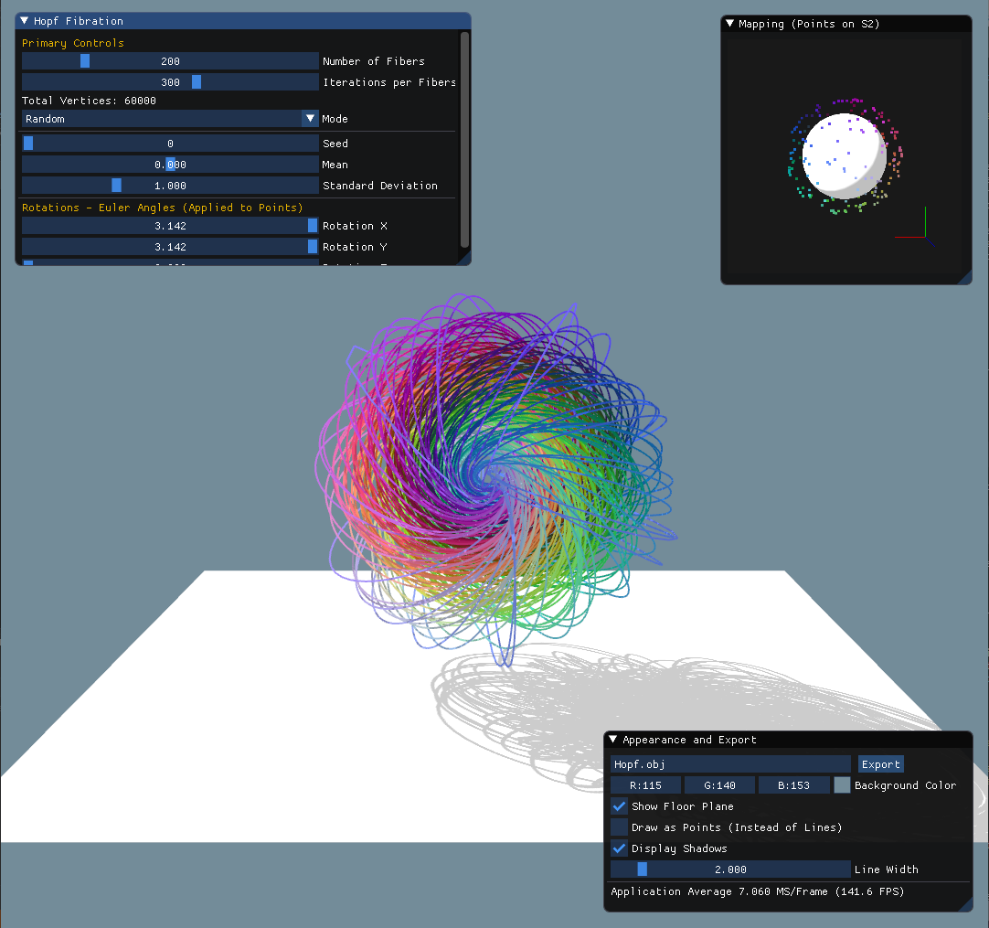
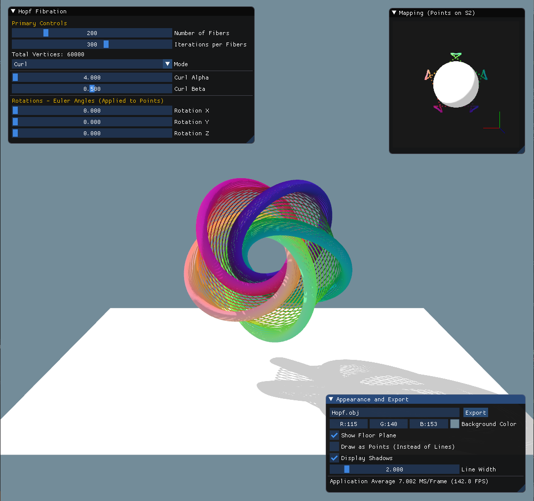
Within the panel labeled “Hopf Fibration”, there are several “mapping modes” available, each of which corresponds to a (configurable) set of points on S2 that form the codomain of the mapping:

• Great Circle: sets the codomain to the set of points formed by one or more great circles on the surfaces of S2
• Random: sets the codomain to a randomly distributed set of points on the surface of S2
• Loxodrome: sets the codomain to a Rhumb line (spiral arc) on the surface of S2
• Curl: sets the codomain to a curled, floral pattern on the surface of S2

Each mode has a specific set of parameters that can be adjusted on-the-fly for changing the fibration. Example images from the four different modes are shown below:

You can use your mouse to rotate the model in space. You can zoom in or out with your scroll wheel. Finally, you can “home” (i.e. reset) the current view by pressing h on your keyboard.

Credits

This project was largely inspired by and based on previous work done by Dr. Niles Johnson, who teaches at Ohio State University. In particular, I used his parameterization of the fibers, as outlined in his production notes. His animated videos of the Hopf fibration are what motivated me to delve into this topic.

Other resources that were helpful during the creation of this project:

• Wikipedia Article on the Hopf Fibration
• Explanation of Quaternions by Ken Shoemake
• A Young Person’s Guide to the Hopf Fibration
• An Elementary Introduction to the Hopf Fibration
• Arcball Cameras
• Guide to Modern OpenGL Functions (DSA)

The shadow mapping code (and many other OpenGL tips) were largely adapted from learnopengl.com, an amazing resource for anyone trying to learn more about the OpenGL API and computer graphics.

back